Machine learning

Dynamic time warping KNN

Note

The source of most of this chapter is http://alexminnaar.com/time-series-classification-and-clustering-with-python.html , which contains a more detailed explanation about the method itself.

A lot of our use cases involve equations around timeseries, which in terms of classification has challenges due to the fact that time is not always aligned.

The default k-nearest neighbor algorithm uses an euclidean distance measurement to calculate the distance of every point in our time sequence, which can lead to odd results when looking at time series.

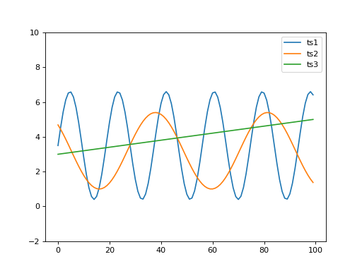
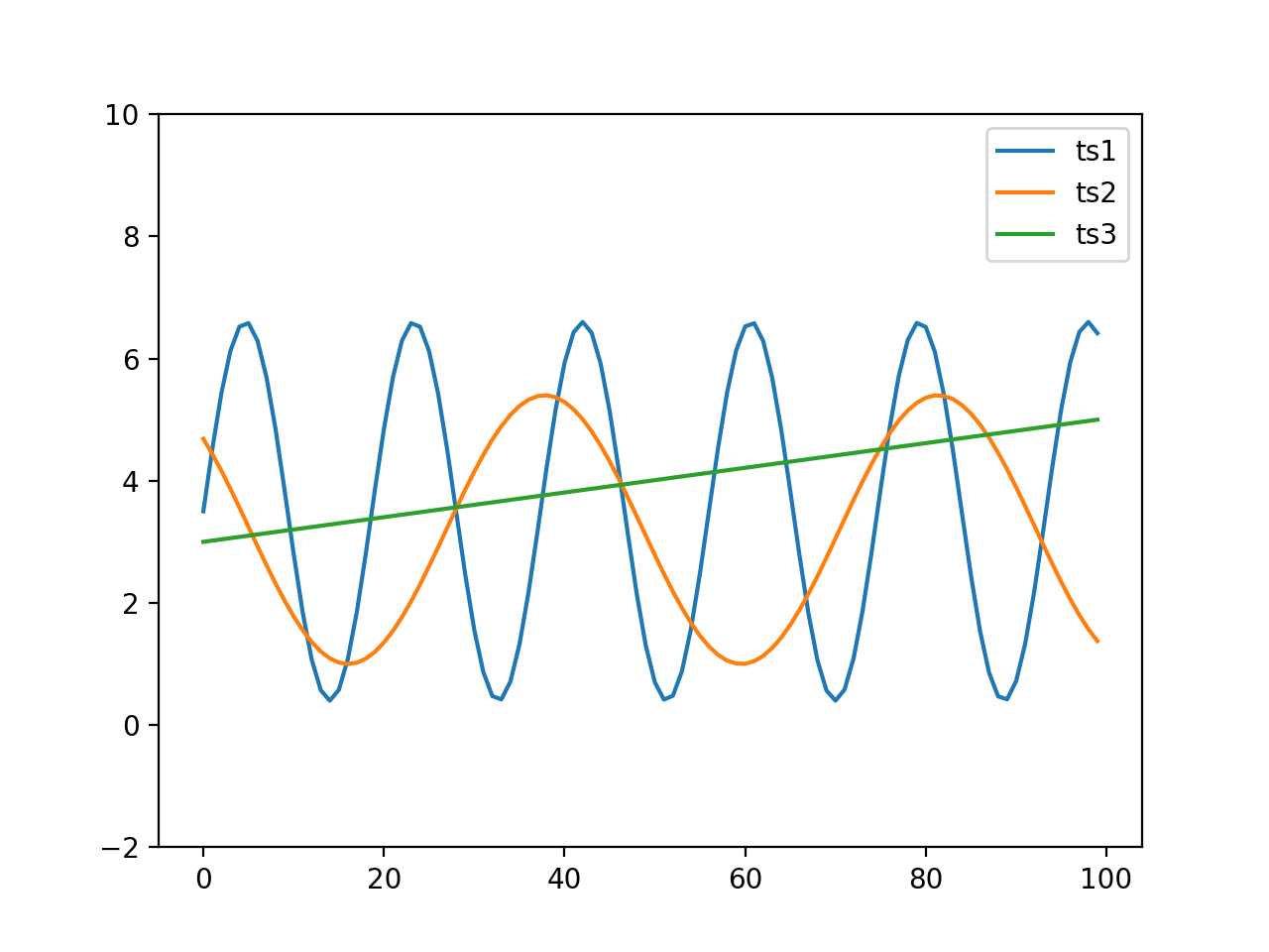
When looking at the following graph, it is clear that ts1 and ts2 are most similar and ts3 is clearly more different. When calculating the distance it would seem otherwise (https://en.wikipedia.org/wiki/Euclidean_distance) sqrt(sum((ts1-ts2)**2)) equals 26.96 and sqrt(sum((ts1-ts3)**2)) equals 23.19.

(Source code, png, hires.png, pdf)

To solve this problem we should actually look ahead or look back in time to find the closest match within certain constraints, which is what dynamic time warping [DTW] can do (https://en.wikipedia.org/wiki/Dynamic_time_warping).

Our framework comes with an implementation of KNN using a DTW distance measurement, which we are going to explain in a couple of steps here.

We generated some data, which can easily be matched to train and test our algorithm.

• input/dtw_train.csv

• input/dtw_test.csv

The code below does a couple of things, the emphasized lines below are about classification and testing, the rest is all about reading, normalizing and displaying our results.

lib_ml_dtw.py

import pandas
import matplotlib.pylab
import sklearn.preprocessing
from valuea_framework.ml import DtwKNN


# read datasets (learn / test data + labels)
datasets = dict()
labels = dict()
for filename in ['dtw_train.csv', 'dtw_test.csv']:
    datasets[filename] = list()
    labels[filename] = list()
    for line in open('input/%s' % filename):
        parts = line.split(',')
        if len(parts) > 1:
            labels[filename].append(parts.pop().strip())
            datasets[filename].append(
                map(lambda x: float(x), parts)
            )

# normalize data
train_dataset = sklearn.preprocessing.scale(datasets['dtw_train.csv'], 1)
test_dataset = sklearn.preprocessing.scale(datasets['dtw_test.csv'], 1)

# train and predict
dtw_knn = DtwKNN()
dtw_knn.fit(train_dataset, labels['dtw_train.csv'])
preds = dtw_knn.predict(test_dataset)
print (dtw_knn.classification_report(labels['dtw_test.csv']))


# use panda and matplotlib to display our data
matplotlib.pylab.figure(dpi=300)
for idx, dataset in enumerate(train_dataset):
    ts = pandas.Series(dataset)
    if labels['dtw_train.csv'][idx] == 'SUS':
        ts.plot(color='red')
    else:
        ts.plot(color='blue')

ts = pandas.Series(test_dataset[0])
ts.plot(color='green', linewidth=3)

matplotlib.pylab.show()

First step is to read our csv data and split our dataset into measurements and labels for both the training and the test set. Next we’re going to scale our data using the scale functions of sklearn.

After training the algorithm with our data and testing it, we are going to output a classification report.

precision    recall  f1-score   support

NRM       1.00      1.00      1.00         5
SUS       1.00      1.00      1.00        10

avg / total       1.00      1.00      1.00        15

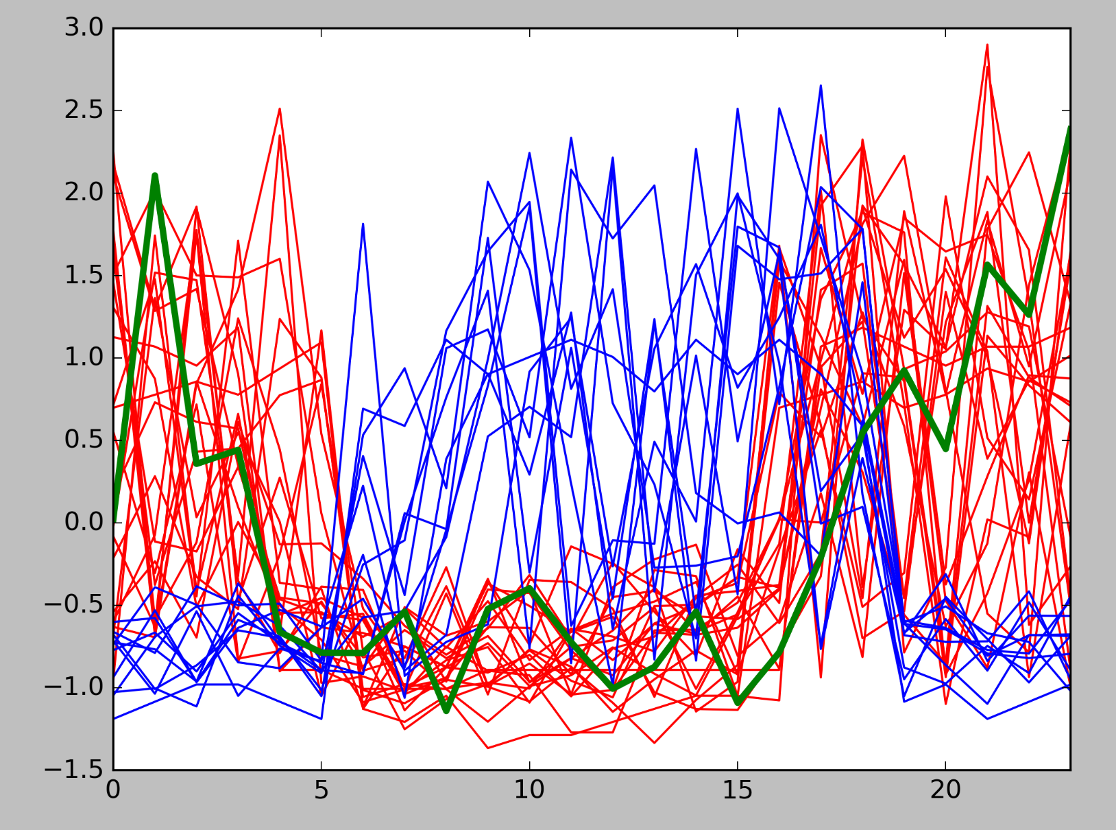
In this case we can see that our test data perfectly aligns to our training set. Using matplotlib we can show our training data and one of our samples, the red lines are suspicious patterns, blue normal and the green thicker line one of our predictions.